Table Of Content
All participants could be tested both while using a cell phone and while not using a cell phone and both during the day and during the night. The advantages and disadvantages of these two approaches are the same as those discussed in Chapter 5. In many factorial designs, one of the independent variables is a non-manipulated independent variable.
Effects and Interaction Plots
Some questions to ask yourself are 1) can you identify the main effect of wearing shoes in the figure, and 2) can you identify the main effet of wearing hats in the figure. Both of these main effects can be seen in the figure, but they aren’t fully clear. We have usually no knowledge that any one factor will exert its effects independently of all others that can be varied, or that its effects are particularly simply related to variations in these other factors. All three of these residuals versus the main effects show same pattern, the large predicted values tend to have larger variation. A transformation - the large values are more variable than smaller values. Well, when we fit a full model it only has one observation per cell and there's no pure way to test for residuals.
Statistical modeling and optimization of heterogeneous Fenton-like removal of organic pollutant using fibrous catalysts ... - Nature.com
Statistical modeling and optimization of heterogeneous Fenton-like removal of organic pollutant using fibrous catalysts ....
Posted: Wed, 30 Sep 2020 07:00:00 GMT [source]
Statology Study
The research designs we have considered so far have been simple—focusing on a question about one variable or about a statistical relationship between two variables. But in many ways, the complex design of this experiment undertaken by Schnall and her colleagues is more typical of research in psychology. Fortunately, we have already covered the basic elements of such designs in previous chapters.
Selecting the Right Factors and Components in a Factorial Design: Design and Clinical Considerations
The following Yates algorithm table using the data from second two graphs of the main effects section was constructed. Besides the first row in the table, the main total effect value was 10 for factor A and 20 for factor B. However, since the value for B is larger, dosage has a larger effect on percentage of seizures than age. This is what was seen graphically, since the graph with dosage on the horizontal axis has a slope with larger magnitude than the graph with age on the horizontal axis. Certainly any research evaluation of intervention effectiveness can pose analytic and interpretive challenges. However, some challenges are of particular relevance to factorial designs.
2.5. Graphing the Results of Factorial Experiments
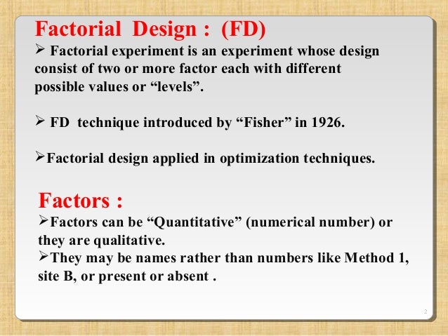
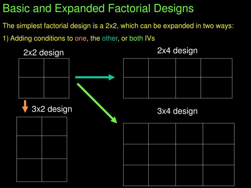
This problem is avoided if an analysis of variance package is used, because such packages typically default to effect coding. In dummy coding, a binary variable, a reference group (e.g., a control group) is assigned a value of zero (0) and the other group (e.g., an active treatment group) is assigned a value of one (1). Effect coding of a binary variable is the same except that the zero for the reference group is replaced with −1. It is also possible to manipulate one independent variable between subjects and another within subjects. To illustrate a 3 x 3 design has two independent variables, each with three levels, while a 2 x 2 x 2 design has three independent variables, each with two levels.
1.2. Measures of Different Constructs
In sum, in a factorial experiment, the effects, relative effects, and statistical significance of ICs will likely change depending upon the number and types of components that co-occur in the experimental design. This arises, in part, from the fact that the effects of any given factor are defined by its average over the levels of the other factors in the experiment. It is important, therefore, for researchers to interpret the effects of a factorial experiment with regard to the context of the other experimental factors, their levels and effects. This does not reflect any sort of problem inherent in factorial designs; rather, it reflects the trade-offs to consider when designing factorial experiments. When taking a general linear model approach to the analysis of data from RCTs and factorial experiments, analysts must decide how to code categorical independent variables.
3.4. What makes a people hangry?
We can look at this two ways, and either way shows the presence of the very same interaction. First, does the effect of being tired depend on the levels of the time since last meal? Look first at the effect of being tired only for the “1 hour condition”.
Just as including multiple dependent variables in the same experiment allows one to answer more research questions, so too does including multiple independent variables in the same experiment. For example, instead of conducting one study on the effect of disgust on moral judgment and another on the effect of private body consciousness on moral judgment, Schnall and colleagues were able to conduct one study that addressed both variables. An example is a study by Halle Brown and colleagues in which participants were exposed to several words that they were later asked to recall (Brown, Kosslyn, Delamater, Fama, & Barsky, 1999)[1].
Factors, Main Effects, and Interactions
If the researcher finds that the different measures are affected by exercise in the same way, then he or she can be confident in the conclusion that exercise affects the more general construct of stress. Once the factorial effects have been computed, the natural question is whether they are large enough to be of statistical and scientific interest. Thus, if all factorial terms are included in the model, traditional regression-based inferences cannot be made because there is no estimate of residual error.
Additionally, a low and high value are initially listed as -1 and 1, where -1 is the low and 1 is the high value. The low and high levels for each factor can be changed to their actual values in this menu. Although the full factorial provides better resolution and is a more complete analysis, the 1/2 fraction requires half the number of runs as the full factorial design.
We have already seen that factorial experiments can include manipulated independent variables or a combination of manipulated and non-manipulated independent variables. But factorial designs can also consist exclusively of non-manipulated independent variables, in which case they are no longer experiments but correlational studies. Consider a hypothetical study in which a researcher measures two variables. The research then also measure participants’ willingness to have unprotected sexual intercourse. This study can be conceptualized as a 2 x 2 factorial design with mood (positive vs. negative) and self-esteem (high vs. low) as between-subjects factors. This design can be represented in a factorial design table and the results in a bar graph of the sort we have already seen.
Traditional research methods generally study the effect of one variable at a time, because it is statistically easier to manipulate. However, in many cases, two factors may be interdependent, and it is impractical or false to attempt to analyze them in the traditional way. You may find that the patterns of main effects and interaction looks different depending on the visual format of the graph. The exact same patterns of data plotted up in bar graph format, are plotted as line graphs for your viewing pleasure. Note that for the IV1 graph, the red line does not appear because it is hidden behind the green line (the points for both numbers are identical). The normal probability plot of the effects shows us that two of the factors A and C are both significant and none of the two-way interactions are significant.
The advantages and disadvantages of these two approaches are the same as those discussed in Chapter 4). The between-subjects design is conceptually simpler, avoids carryover effects, and minimizes the time and effort of each participant. The within-subjects design is more efficient for the researcher and help to control extraneous variables. This would mean that each participant would be tested in one and only one condition. This would mean that each participant would need to be tested in all four conditions. The advantages and disadvantages of these two approaches are the same as those discussed in Chapter 5.


No comments:
Post a Comment